Disclaimer

This article is built entirely on my understanding and mental model of the Go Scheduler, CFS and CPU clock cycles. I’ve tried to validate everything based on external sources but If I have made a mistake or something is not entirely accurate then feel free to shoot me a message on LinkedIn 🙂

Introduction

This article was starting to get a bit long, still is pretty long 😅 so I have decided to break it into 3 parts:

• Pt 1 Building a mental model.
• Pt 2 Understanding your tools.
• Pt 3 Putting it together with benchmarks.

So what is P99? It is the 99th percentile of distribution or in latency terms it means 99% of request/response times finish within this time. For example if a web servers P99 latency was 3 seconds and we measured 100 requests then out of those 100 requests 99 would return in 3 seconds or under. Chasing an improved Tail Latency - anything above P90 can be a long road and further drilling down into P99 can be an even longer, winding road filled with detours and dangerous obstacles along the way ⚠️. It’s no small challenge tackling P99 but optimising for the 1% of users that experience these slow latencies can make big impacts at scale. For example back in 2006 Amazon found that for every 100ms added to page load times resulted in them losing ~1% in sales. The 1% of users that were experiencing these large page load times lead to users abandoning their carts and not coming back which lead to approximately $107 million in sales left on the table that never converted!!

Hopefully in this three part series I’ll arm you with the insight and tools you need to sculpt a high performance Go application. Just as a master sculptor understands the grain of their medium and the precise impact of every chisel strike to craft a masterpiece, we must understand the “material” of the underlying systems we work on top of.

In Part 1 we will delve into the Go scheduler, Linux Scheduler and part of the CPU to help build a mental model of how these systems cooperate. Developing this clarity will hopefully give you the technical depth required to solve the kind of complex problems that remain unreachable without a deep understanding of these systems.

A look under the hood - The Go Scheduler

If you have worked with concurrency in the past (coroutines in Kotlin and goroutines in Go) you may be familiar with the different multi threading models. There’s typically three models many-to-one (N:1), one-to-one (1:1) and many-to-many (M:N).

Go opts in for the many-to-many (M:N) model which provides a high level of concurrency because if one thread blocks another can continue where with a many-to-one (M:1) if one thread blocks then it blocks the entire process. With one-to-one there is no blocking of the other threads If one thread decides to block but the overhead is higher compared to many-to-many because each user thread ie: goroutine requires a corresponding OS Thread thereby making the M:N model a great fit for the Go Scheduler.

The Go scheduler is part of the Go runtime and its main responsibility is the orchestration and running of goroutines which are lightweight application threads starting at 2KB in size as defined by stackMin. We can create a new goroutine by using the go keyword followed by a function call. Every new instance of a goroutine contains metadata such as the execution state, stack and program counter pointing to the associated function.

When we spin up a new Go application the runtime will reach out to the machine (virtual or physical) and identify how many cores there are. It will then use this number to create its own internally managed logical processors to represent these cores via a struct p, which we will refer to as P. For every P or logical processor that the scheduler manages it will own its own OS Thread or machine Thread which is controlled by by struct m, which we will refer to as M. The struct m holds a reference to the current goroutine and the current logical processor P if the M is executing go code.

The best way to think about the P is that it acts as the middle man or bridge between our go application and the OS.

Now the Go scheduler is responsible for the orchestration of goroutines which are managed by struct g, which we will refer to as G. So what the scheduler will do is take these goroutines (G’s) and assign them a P where the P will then run the G on an M (machine thread). This means that for each logical processor P we can have at most 1 M and for each M it can be running at most 1 G. Its a 1:1:1 ratio. This is referred to as the GMP Model.

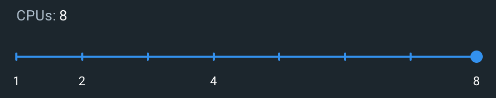
For example if I were to bring up the system report of my MacBook and inspect the number of cores, you would see that I have a total of 8 cores. This would result in my go application having a total of 8 P’s there by allowing me to run 8 goroutines in parallel. If your a coffee fan thats kind of like having 8 gophers all making coffee at the same time!!!

Goroutines are similar to OS Threads in the sense that like OS threads which can be context switched on/off a core a goroutine can be context switched on/off a M. Though a goroutines lifecycle is much simpler than an OS thread and it can be in one of 3 states:

• Executing → The goroutine has been placed on a M and is executing its instructions.
• Runnable → The goroutine is waiting to be in an executing state.
• Waiting → The goroutine has been moved off the M and is placed in a waiting state. This usually happens when the goroutine has to perform some IO or synchronisation like acquiring a mutex.

So I said there were just 3 states…. I lied. There are actually a couple more which are not as significant as the main 3 but worth mentioning:

• Idle → goroutine created but not initialised.
• Syscall → Executing a system call and not running go code.
• Dead → The goroutine is in what is called the free list.

I just want to quickly touch on the the Dead state because this is partly why goroutines are so optimal. When a goroutine finishes executing it is dead 🪦 and is placed into what is referred to as the free list. This will either be the local free list of the P or a global free list. When a new goroutine is created it will try to recycle an old goroutine from the free list otherwise it will spin up a new one. This recycling process ♻️ is what makes goroutines so cheap to create!

Now if a goroutine is the main path of execution and if your spinning up multiple G’s more than the number of P’s that are available then what happens to those G’s? Well short answer is queueing.

When a goroutine has no place to go it is placed on either the runq (a local fixed size circular queue of goroutine pointers) which is managed by a P or the global queue. The fixed size queue of 256 is sufficient enough for a local queue and the circular structure which uses the ring buffer algorithm enables the adding and removing of goroutines in constant time O(1) without the need to shift the array.

So what happens in the case above where M1 has moved the G off the OS Thread and doesn’t have a G to run? The answer is stealing! The go scheduler is referred to as a work stealing scheduler. What this means is that if an M is free then the P can look out to the global queue and other P’s local queues and if it sees a G in either of these queues it can steal it and place it on it’s M. This allows for an under-utilised P to find work.

Lastly in the early days of Go prior to Go 1.14 if a goroutine had a tight loop performing cpu bound work (i’ll touch on cpu bound work later) then the thread would hold on to this goroutine until all the work was completed there by creating a backlog of goroutines which had nothing to do but sit idle waiting for this long cpu bound task to complete. Us Gophers could get around this by using runtime.Gosched() in the body of the loop though this was very tedious and error prone and did have some perf issues. More details on this here → runtime: tight loops should be preemptible #10958.

Though in Go 1.14 the Go team decided to move away from a cooperative scheduler and instead moved to a preemptive scheduler which solved a lot of these issues. At a high level Go runs a daemon on a dedicated thread M called sysmon (system monitor) which is not attached to any P. When sysmon finds a goroutine that has been running for longer than 10ms as defined by forcePreemptNS it sends a tgkill signal (the name is misleading. It does no killing just sends a signal to the process ✉️) to the M running the goroutine. The goroutine will then be suspended and put into the global run queue where it will be later picked back up by a P. This then frees up other goroutines to do work ensuring a fairer balance of goroutine time on the OS Thread.

Go’s I/O Model

To understand how Go handles IO we need to take a look at blocking, non-blocking and multiplexing IO.

With your typical blocking IO operations a thread will suspend or pause until the system is ready with the requested data. On the other hand non-blocking IO does NOT suspend and the Linux Kernel will return the requested data if its there or an error EAGAIN or EWOULDBLOCK which are two error codes that share the same value as outlined by POSIX.1-2001 that signify Resource temporarily unavailable.

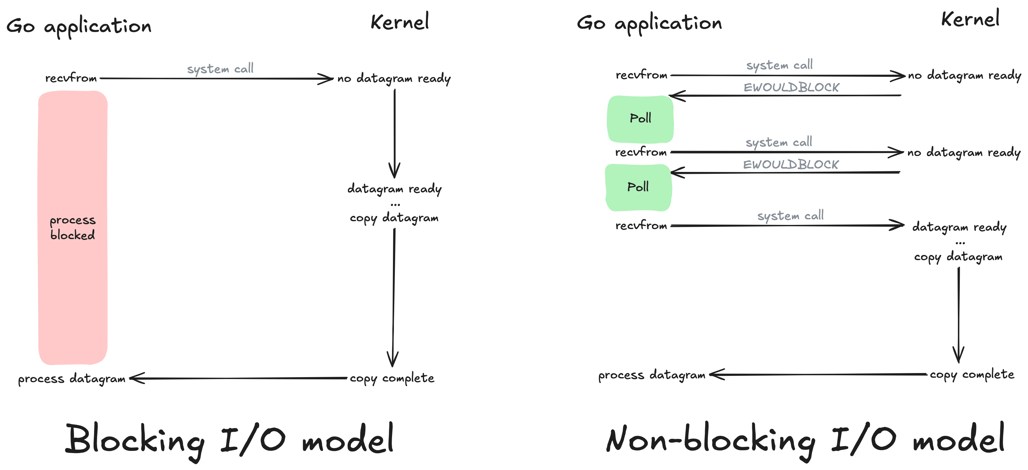
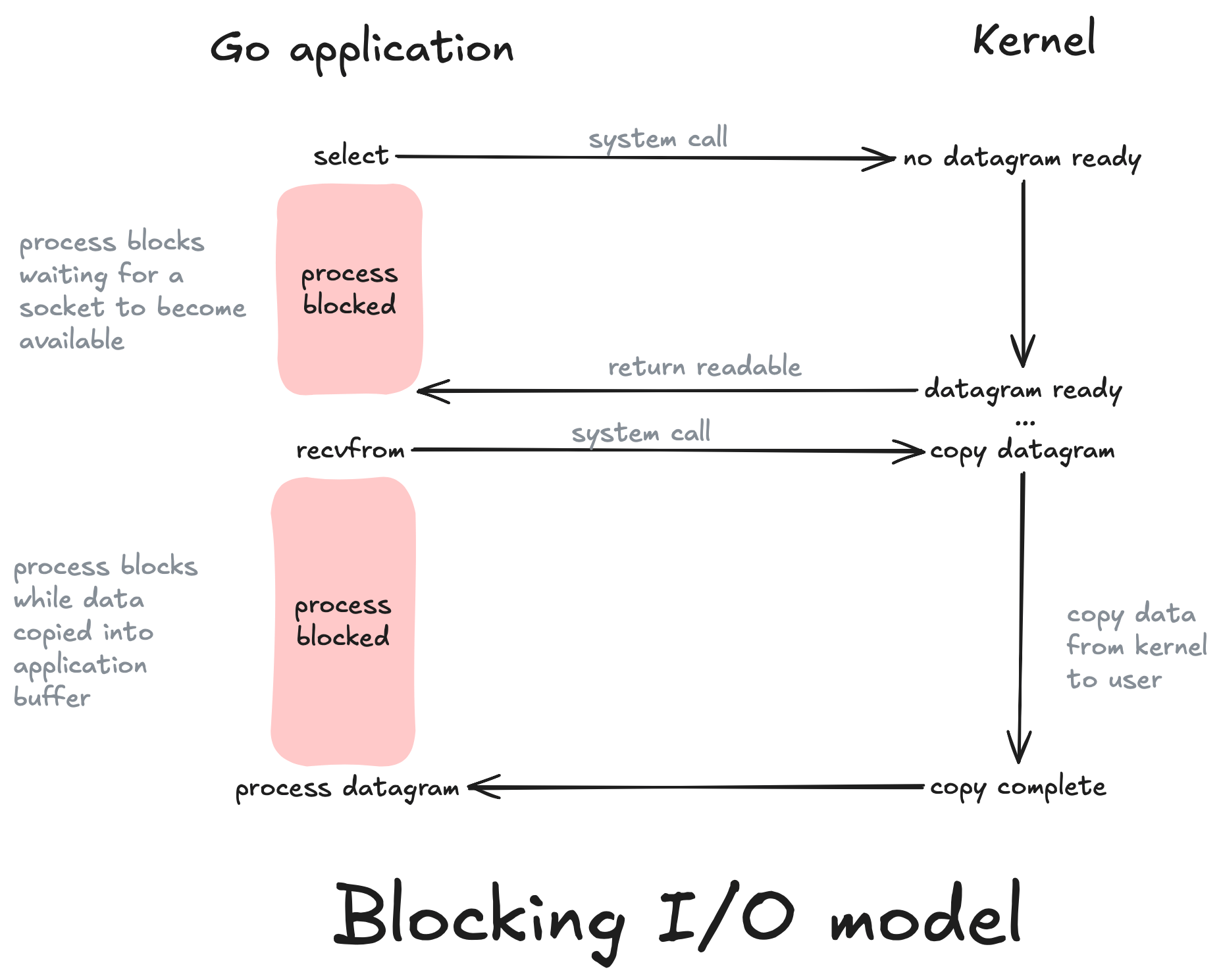
In I/O Multiplexing a combination of select() and poll() system calls are used for monitoring multiple file descriptors that will later become ready to perform I/O. Our application will block on one of these system calls rather than on recvfrom as used by blocking and non-blocking models. The multiplexing model uses select to notify our application that a socket is readable in which case our application can then make the system call via recvfrom.

Go uses a combination of non-blocking and multiplexing models to handle I/O efficiently but select and poll are extremely inefficient in comparison to Linux epoll. Linux epoll is an API (epoll_create, epoll_ctl, epoll_wait) that is used to monitor multiple file descriptors to see if they are ready for I/O.

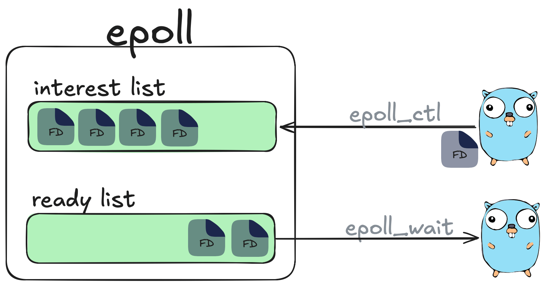
From the users perspective epoll contains two lists:

• The interest list which contains a set of file descriptors the process has registered an interest in monitoring which can be registered via epoll_ctl.
• The ready list which contains a list of those file descriptors we are interested in that are ready to perform I/O. We can monitor this list via epoll_wait which will block the calling thread if no events are currently available.

A single thread using epoll can handle tens of thousands of concurrent requests and is a lot more efficient in comparison to other mechanism’s such as poll and select as shown in the following experiment from the book Linux Programming Interface.

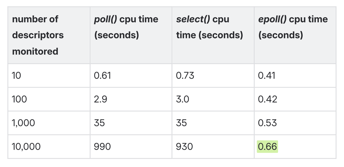Table taken from pg 1365 of The Linux Programming Interface by Michael Kerrisk.

What I love about the Go scheduler is its ability to leverage Linux epoll.

If a Goroutine needs to perform a network based system call then Go has the ability to move this G off the M and place it in what is called the Net Poller which in turn registers the file descriptor using epoll_ctl with EPOLL_CTL_ADD. This then prevents the goroutine from blocking the M and frees it up to run another goroutine.

Go’s net poller then uses the epoll_wait system call to then collect batches of 128 where it then cycles these events back to the go scheduler.

Lastly it’s important to clean up these file descriptors to avoid starving a goroutine. This is done by calling epoll_ctl with EPOLL_CTL_DEL operation which will unregister the file descriptor in the epoll interest list.

What is clever about this approach is that this moves the hard work of processing network requests from the scheduler to the OS.

Prior to Go 1.25 any P could use the net poller instance but for workloads that were leveraging a large number of cores this lead to serious cpu time spent on epoll_wait so as part of Go1.25 the netpoller is only polled from a single thread in order to avoid kernel contention → runtime: only poll network from one P at a time in findRunnable

If your also interested there are talks of potentially using io_uring for doing file I/O. If you are interested you can read about it in the paper Efficient IO with io_uring or if you want to follow the discussion on GitHub you can go here internal/poll: transparently support new linux io_uring interface #31908.

Diving one level deeper - The Linux OS Scheduler

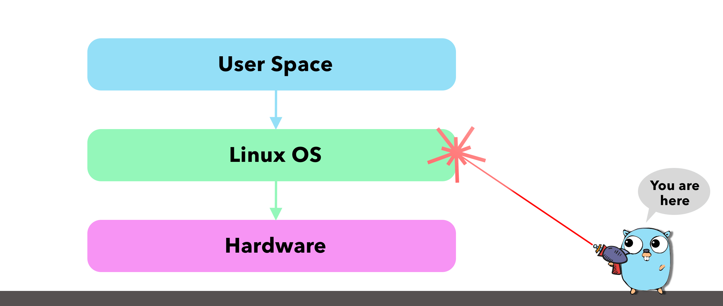
Our Go Scheduler uses a OS Thread (M) to run its goroutines but what is the M really? Threads are the smallest unit of processing an OS can perform. They are responsible for executing instructions on the hardware. Every process running on our machines is allocated at least 1 thread with the ability for this thread to spawn more threads.

Similar to our Go Scheduler an OS Thread can also be in 3 states:

• Executing: The thread is placed on a core and is running its instructions.
• Runnable: The thread is is hanging out and waiting to be executed.
• Waiting: The thread was running but has been stopped and is now waiting to be placed on a core again.

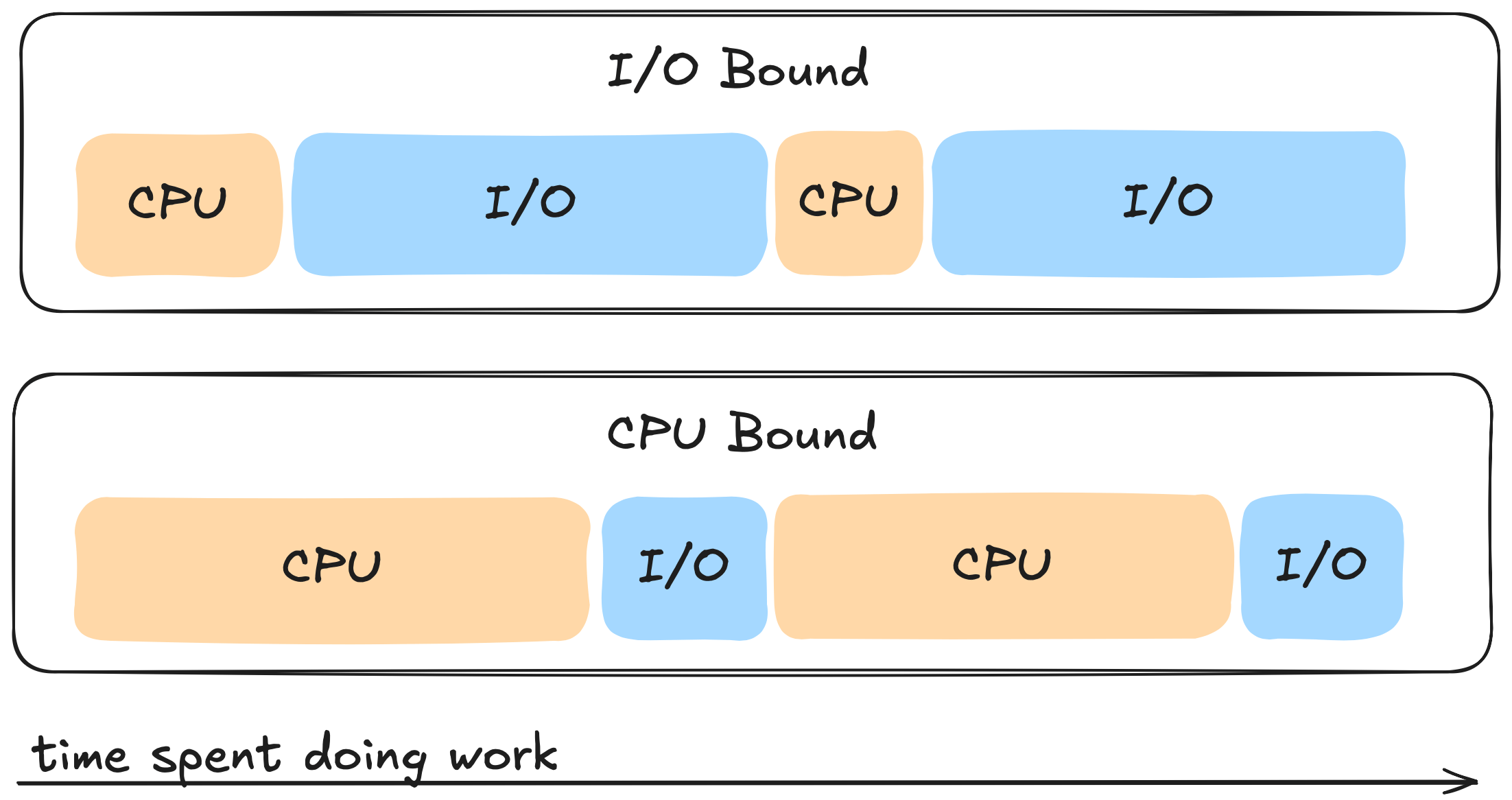
Each Thread can perform two types of work:

• CPU-Bound: This is work that results in the thread never being able to be placed into a waiting state and often times involves some sort of calculation like calculating the nth Fibonacci number.
• IO-Bound: This type of work on the other hand can cause the thread to be placed into a waiting state and often times involves performing:
  • Network calls
  • System calls
  • Synchronisation events, things like atomic operations and mutexes.

If a thread has a lot of cpu bursts when compared to IO work then we refer to this as a cpu bound task. If a thread on the other hand is mostly doing IO work then we refer to this as a I/O bound task. Its good to know what category your application falls under as this can help steer us in the right direction when it comes to fine tuning our go applications.

When it comes to scheduling these tasks there are two main approaches the OS can take. The first is cooperative where a task comes in we can either pick it up or pick up another task that’s been waiting to run. We then place that task on the cpu and run it to completion then when its done it makes a system call and gives up the cpu cooperatively so the next task can then run its instructions to completion on the cpu.

The Linux OS on the other hand uses a Preemptive Scheduler which involves interrupting a task when it has exceeded its allocated time (quanta/time slice) and taking the thread that is in the Executing state and moving it to the Waiting state so the OS can then take a higher priority task and move it from either the Runnable or Waiting state to the Executing state. Hey Hey Hey this sounds kind of similar to the Go Scheduler right! 🧐 This type of scheduling however makes it next to impossible to predict what actions the scheduler will perform.

This action of moving Threads on and off a core is referred to as a Context Switch and is considered to be an expensive operation - especially at the OS level. The size of an OS Thread on Linux is ~ 2MB on Linux/x86-32 which is about 1000x the size of our goroutine - the larger the thread size the more expensive a context switch can be. There are other factors at play that can affect how expensive a context switch can be but it wouldn’t be unreasonable to say that a single context switch can take approximately 1000-1500 nanoseconds. Doesn’t seem like much but boy o boy as you’ll see later it can be!

The Linux Scheduler along with being preemptive is also a priority based scheduler meaning it will pick the highest priority task in the highest scheduling class. The lower the priority value the higher up on the chain the task is in terms of being prioritised.

There are two types of scheduling classes. The first is **Real-time_**which involves the use of FIFO or Round Robbin of tasks running to completion or until they exhaust a time slice. This class has the highest priority and is often reserved for high priority tasks.

The second class is Normal class which uses Completely Fair Scheduler (CFS). This is where we will be focusing most of our time and later on in Pt2 and Pt3 we will see how we can optimise CFS to help reduce the tail latency of our Go applications.

CFS is a process scheduler developed by Ingo Molnár and merged in Linux 2.6.23. In a nutshell it is a way in which the Linux OS ensures that every process gets its fair share of resources (cpu, memory etc…) and no one particular process is hogging all the resources.

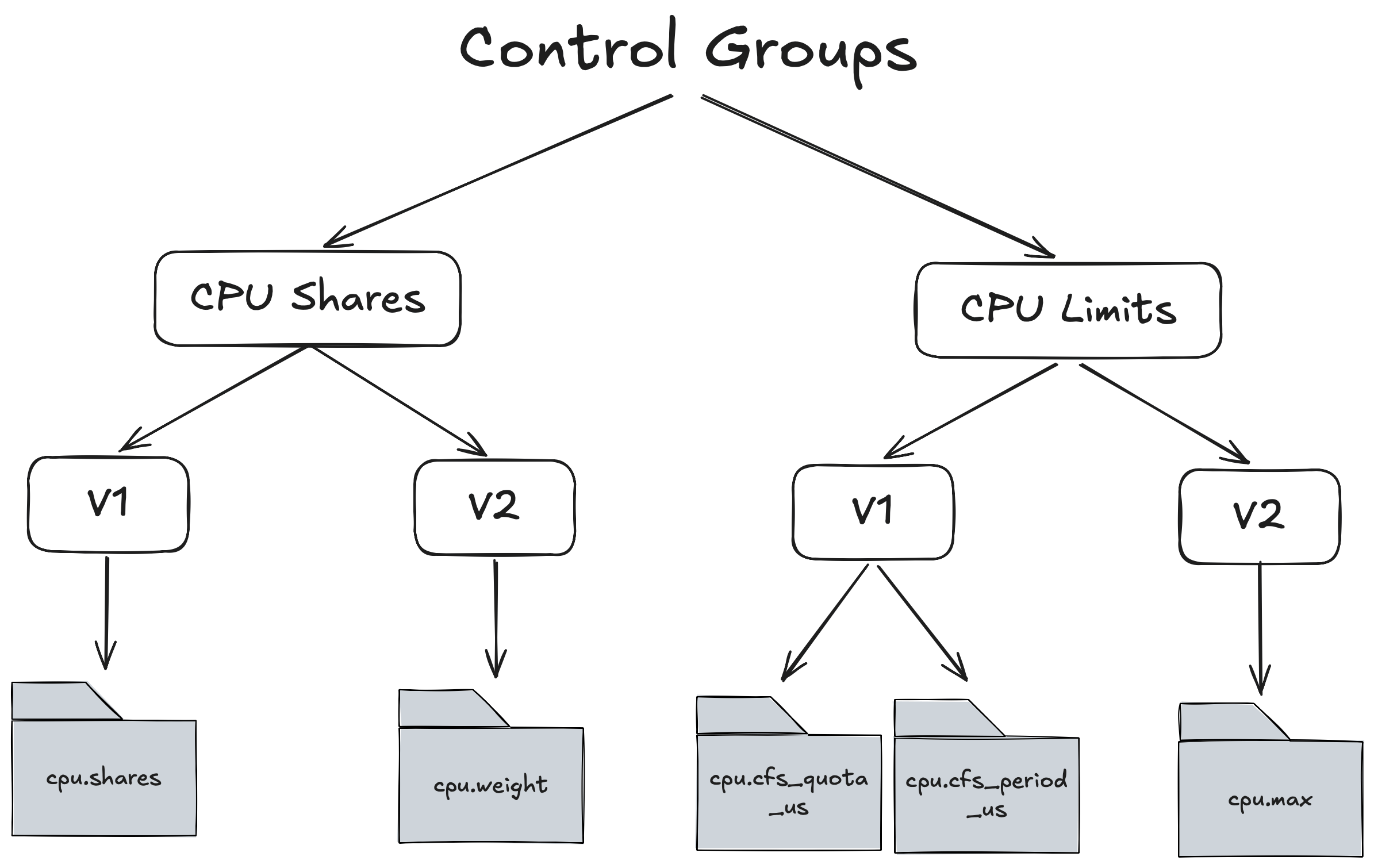
The main system resource we will be focussing on in this article is CPU. The way in which we can tell a particular process how much CPU it is allowed to consume is through Linux Control Groups which are part of CFS. There are 2 main control groups for allocating CPU and for each control groups there are 2 versions V1 and V2.

Lets start with CPU Limits but before we dive in it’s important to understand that when we allocate cpu to a process we are NOT allocating a whole or part of a cpu but what we are in fact allocating is the amount of time that process gets on the cpu ⏱️.

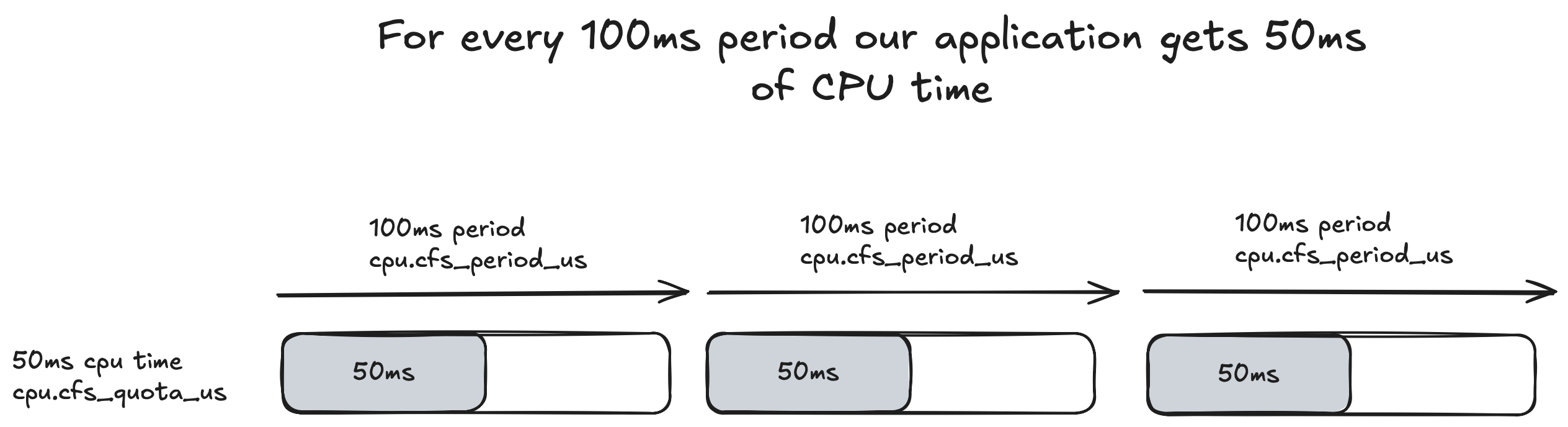
How does this time based allocation work exactly? For CPU Limits the Linux OS runs a constant 100ms cycle that keeps iterating indefinitely. This is referred to as the CPU Period and can be configured via cpu.cfs_period_us in V1 or in cpu.max for V2 and is a global setting.

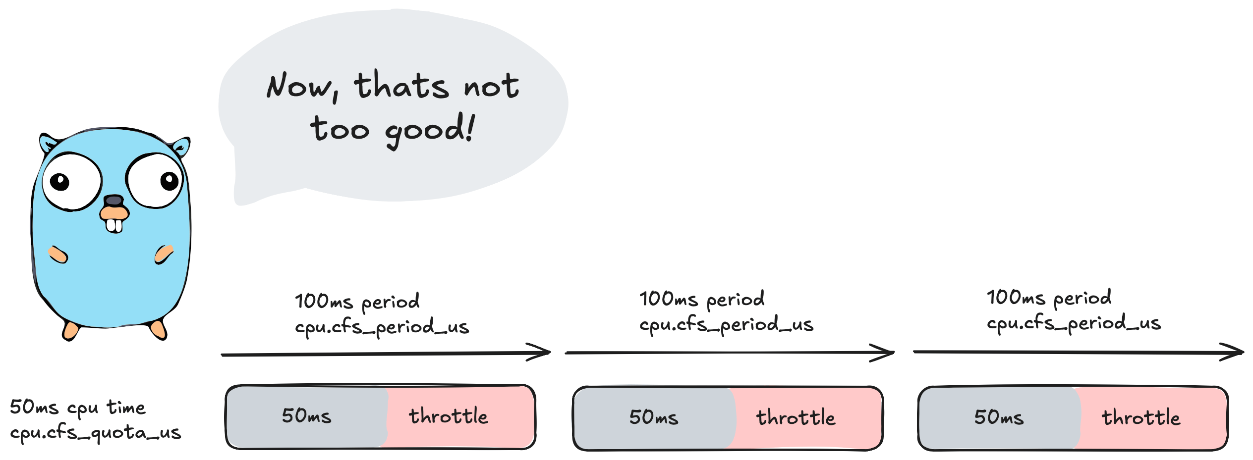
For each 100ms period we can allocate the amount of CPU Time/Quota this process gets to run. This can be configured via cpu.cfs_quota_us.

For example if we had a single threaded application that we gave 50ms of cpu time then we would set it like so:

cpu.cfs_quota_us = 50000

This is set in milliseconds. An illustration of how the quota works in relation to the period is show below:

If we cat these files for control groups V1 we get:

cat /sys/fs/cgroup/cpu,cpuacct/cpu.cfs_period_us // 100000

cat /sys/fs/cgroup/cpu,cpuacct/cpu.cfs_quota_us // 50000

And for control groups V2:

cat /sys/fs/cgroup/cpu,cpuacct/cpu.max // 50000 100000

So the question then is what happens once we reach this 50ms cpu time? The answer is

🚨🚨🚨Throttling🚨🚨🚨

At 50ms of cpu time CFS will step in and stop/throttle ✋ our application for the remainder of the 100ms period. So in this scenario here our application would sit idle for 50ms doing absolutely nothing.

We can also inspect this behaviour by looking at the cpu.stat file.

Here is a stat ripped from Uber/automaxprocs experiment where a quota of 2 cpu was set on a 24 core machine. The large variance of quota and cores is to emphasise the throttling.

  cat /sys/fs/cgroup/cpu,cpuacct/system.slice/[...]/cpu.stat

  nr_periods 42227334
  nr_throttled 131923
  throttled_time 88613212216618

• nr_periods represents the total number of control group periods that have elapsed since the control group creation.
• nr_throttled is the number of times the process was throttled.
• throttled_time is the amount of time our app was throttled and sitting idle and not able to perform work.

If we do some basic maths we can work out how long this experiment ran for:

(42227334 * 100ms) /1000/60/60/24 = 48 days this control group ran for.

and how much time our application was spent throttled:

88613212216618 / 1000ns / 1000µ / 1000ms / 60 / 60 / 24
~= 1 full day of throttling out of 48 days of running.

If this was scaled up to a year that would be approximately 1 whole week where our application was doing 𝟎, nada, nil, zilch work. Thats like our application deciding to take a full week off work.

CFS provides us with another control group mechanism we can use to configure resources for our tasks called CPU Shares.

CPU Shares act a bit different to CPU Limits. There is no concept of a 100ms period and instead we go off wall time (elapsed real time) 🕗. We also no longer allocate an exact amount of cpu time to a process but instead give each process a weight that we can use to distribute how much cpu time each process gets. To help explain this I’ll give two examples.

Example 1.

If I have 2 processes (A and B) running side by side and each process is given a equal weight of 512:

CPU Time A = A / (A+B)

CPU Time B = B / (A+B)

CPU Time = 512/(512+512) = 50% cpu time.

Process A and B would get roughly around the same amount of time on the CPU.

Example 2.

Process A is given a weight of 768 and Process B = 256

Process A CPU Time = 768/1024 = 75%

Process B CPU Time = 256/1024 = 25%

Process A now gets 3 times the amount of CPU time compared to process B.

In control groups v1 we can configure the weight via cpu.shares:

cat sys/fs/cgroup/cpu,cpuacct/cpu.shares // 1024

In control groups v2 we set the weight via cpu.weight and setting a similar weight would display:

cat sys/fs/cgroup/cpu,cpuacct/cpu.weight // 39

This is because in control groups v2 the weight is based off of the following formula:

cpu.weight = (1 + ((cpu.shares - 2) * 9999) / 262142)
= (1 + ((1024 - 2) * 9999) / 262142) ~= 39

This conversion does come with a few problems for k8s workloads 🙊 which are outlined in New Conversion from cgroup v1 CPU Shares to v2 CPU Weight

This means that as time passes the Linux OS will try to balance the cpu time based on the percentages we calculated.

Here’s the thing though. These weights really only take effect when the processes are under contention ie: battling for more cpu time ⚔️. In the case of example 1 and 2 if process A is sitting idle and isn’t using all of its cpu time and process B is under heavy load and needs more cpu time it can then use all of the cpu time not used by process A. Its worth repeating that this only happens under contention.

Question though, if time is progressing based off of wall clock time how does CFS ensure each process gets its fair share of cpu time relative to its weight?

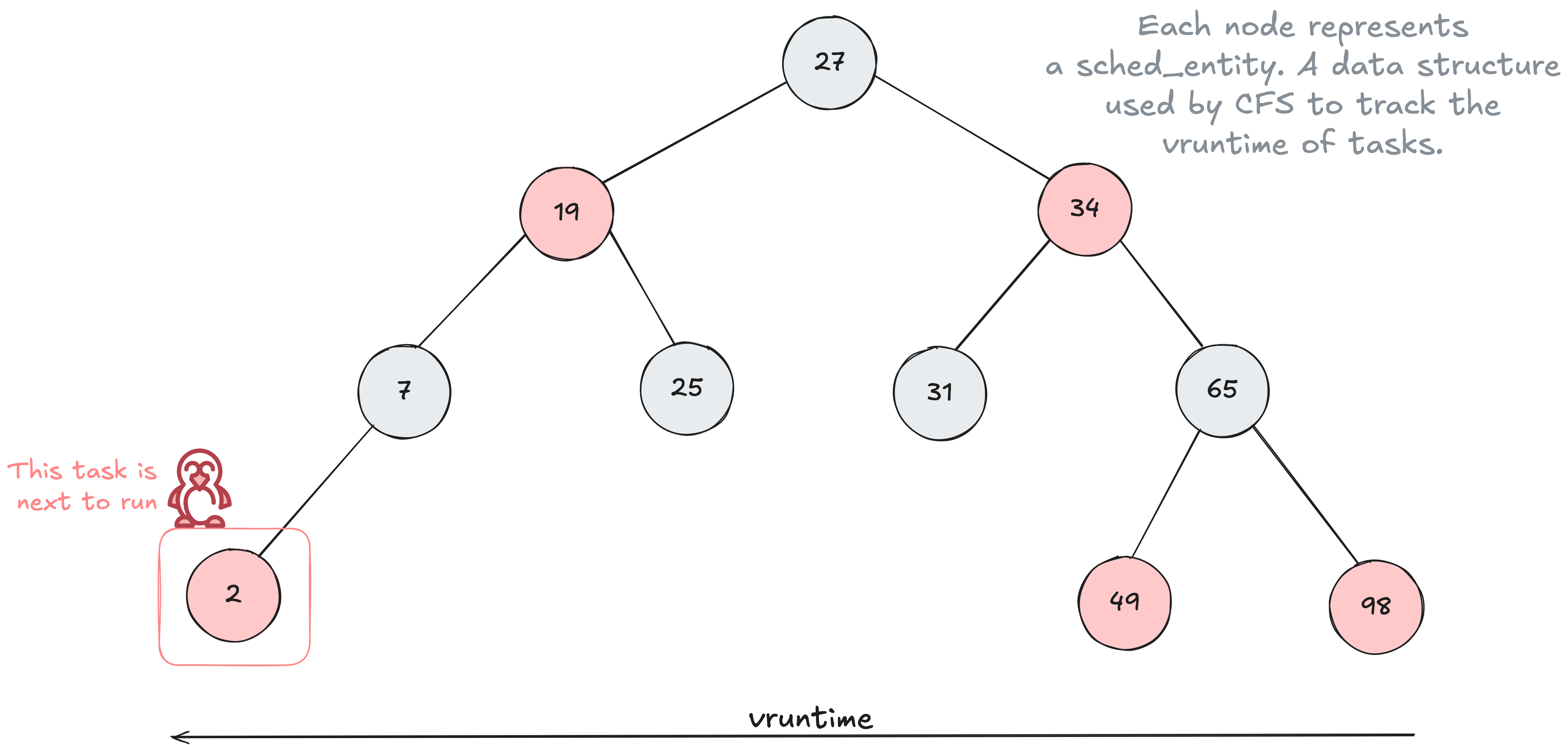
The answer is through the use of a time ordered Red Black Tree 🌳 data structure to help build a timeline of future task execution. Every task that is placed into the tree is sorted based on their vruntime key. The vruntime is a value that keeps track of the amount of time that task has run on the cpu.

As time progresses forward the tasks are put into the tree more and more to the right with these tasks slowly making their way to the left side of the tree. CFS will then select the left most task in the tree to run next.

The ordering of the tree is based on having tasks with smaller vruntime to the left of the tree and larger vruntime to the right. A smaller vruntime means the task has had less time on the CPU.

The vruntime value can be altered through the use of CPU Shares. Tasks with a higher weight have their vruntime change at a slower pace 🐌 there by moving them further left 👈 in the tree more often compared to tasks with a lower weight which increases the vruntime at a faster pace 🏎️ keeping the task further right 👉 in the tree.

The formula for calculating the vruntime based on control group weight can be shown below:

vruntime += actual_task_runtime ×(1024 / weight)

Every time a scheduler tick (not to be confused with a clock tick) is performed the tasks CPU usage is accounted for and the vruntime is recalculated until it is no longer the left most task and another task is selected.

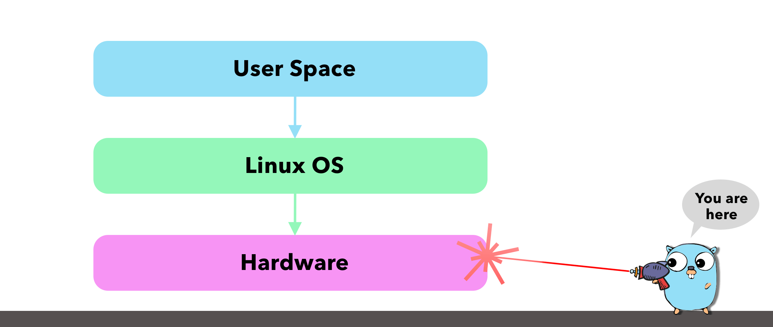
Diving two levels deeper - The clock cycle of a CPU

There are many aspects of a CPU we can focus on and drill down into - too many for a single blog post. Instead, I wanted to focus on the clock cycle and try get an understanding of how time correlates to instructions so we can see how an incorrect scheduler setup directly leads to missed instructions.

The CPU clock speed is the tempo your processor runs at or the number of ticks it can perform per second, similar to a heartbeat. It’s often measured in hertz (Hz) and on modern day CPU’s you’ll see gigahertz GHz which are billions of cycles that coordinate what instructions the cpu performs next or in biological terms this is like billions of heartbeats per second.

3.6 GHz = 3,600,000,000 cycles per second

= 1 / 3.6*10^9 = 0.000000000277778 seconds per cycle or

= 0.000000277777778 milliseconds per cycle or

= 0.000277777778 microseconds per cycle or

= 0.277777778 nanoseconds per cycle

1 tick or 1 cycle therefore takes only ~0.278 nanoseconds on a 3.6GHz CPU. Note that every cpu is different and this is just a gauge to go off as the microarchitecture varies from cpu to cpu. For example a modern M1 processor running at 2.5GHz is plenty times faster than an old school Pentium 4 Processor running at 3.8Ghz.

So, what does this mean for us? Take an Intel i7 running at 3GHz as an example. That speed translates to 3 clock cycles every single nanosecond. If that CPU performs 4 instructions per cycle, it’s processing roughly 12 instructions per nanosecond.

An instruction in simple terms is just an order given to the computer processor by the computer program or in our case its our Go program telling our CPU to do something.

So if we move back up the chain to the OS level where we utilise threads to perform these instructions we mentioned earlier that moving the thread on/off the core ie: context switching the M took around 1000 nanoseconds or in our case this is a whopping 12,000 instructions that we just missed out on because of a context switch that our program could have been performing otherwise.

A goroutine which if we recall are light weight application level threads that run on the thread take ~ 200 nanoseconds to be context switched on/off the M. Therefore we only lose ~2,400 instructions when we context switch at the application level vs the OS level. This is a difference of ~9,600 instructions 🤯

This becomes even more evident when using CPU Limits. In our previous example, we set a limit that caused the application to throttle for 50ms. Since our CPU can handle 12 million instructions per millisecond, that 50ms gap represents 600 million potential instructions our application missed out on during that single 100ms period 🤯🤯 (double exploding head!)

I guess now when we look at it like this a few milliseconds can mean a lot of work our application’s could have been doing otherwise.

Starting our Go application for the first time

Now that we have a bit more of an understanding from the Go Scheduler level down to the OS and CPU I want to close out this article by looking at how our Go program can configure the number of P’s which in turn sets the number of M’s and therefore the number of goroutines we can run in parallel.

In Go we have this nice little function and environment variable that is part of the runtime package which is responsible for setting the number of operating system threads M’s that can run user level go code. This function / env variable I am talking about is GOMAXPROCS.

We can manually set the number of P’s via env variable:

GOMAXPROCS=5 go run .

Or In our Go application code:

runtime.GOMAXPROCS(5)

We can get the current value for gomaxprocs by passing 0 to the function:

fmt.Println(runtime.GOMAXPROCS(0)) // prints 5

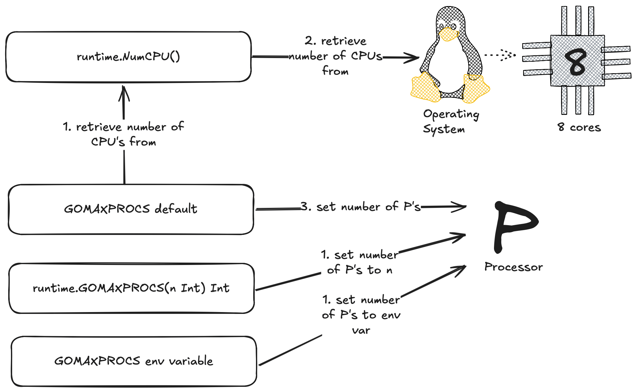
A lot has changed for gomaxprocs in Go version 1.25. In version 1.24 when our application booted up for the first time the Go runtime would try to figure out what to set for GOMAXPROCS by asking runtime.NumCPU() what the value should be. The runtime.NumCPU function would look at the number of cores on the machine and set this for GOMAXPROCS.

Now this could be problematic for a lot of Go users because if your like most people your probably running your Go applications in Docker and using some form of container orchestration like Kubernetes.

For example here is a K8s Pod with 8 cores and a container with a hard limit / cpu limit of 4. Now if your not aware Kubernetes uses CFS to enforce these limits so what would happen in go apps running go 1.24 or lower is the following:

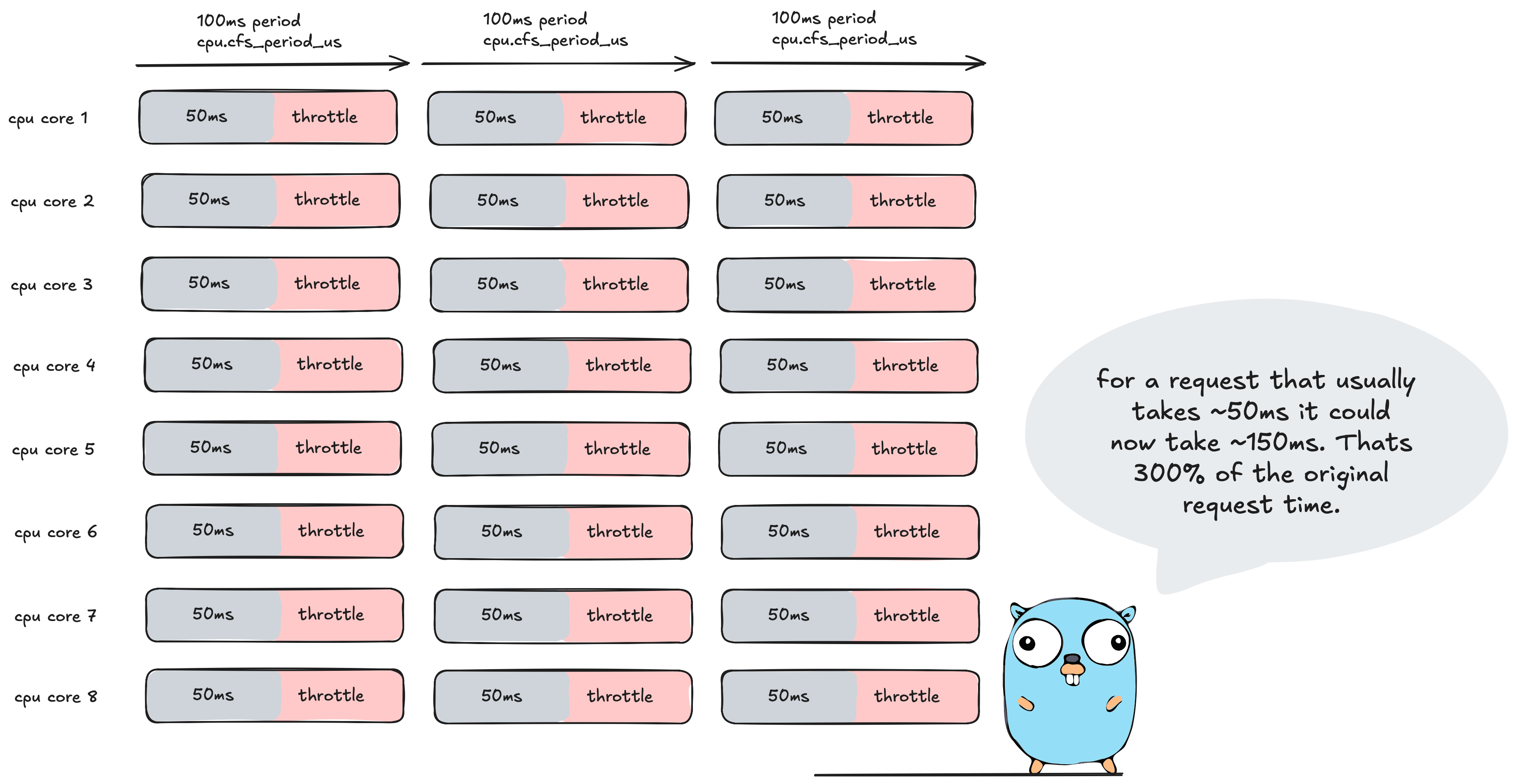
runtime.NumCPU() returns 8 cores which sets the max parallelism to 8. Now if you recall we set the limit to 4 which in turn sets the cpu.cfs_quota_us to 400ms which is 400ms of cpu time per 100ms period.

So what happens to our Go application? Each OS thread is going to run go routines for ~50ms.

Why only 50ms you say? If we add up each threads cpu time, that is 50ms x 8 threads = 400ms of cpu time which equals the cpu limit set by the container. This results in our Go application then being throttled for the remainder of the period. Oh dear me 🤕

In Go 1.25 this issue was addressed by making the Go Scheduler CFS aware. This was big news for us K8s devs who were use to using uber/automaxprocs to solve the infamous #33803 issue.

So lets dive in and have a look under the hood at how the Go team addressed this issue.

In terms of the functions and environment variables available to us for setting GOMAXPROCS, it is relatively the same except now we have a new function called setDefaultGOMAXPROCS() which is available to us if we ever want to revert back to the default implementation outlined below.

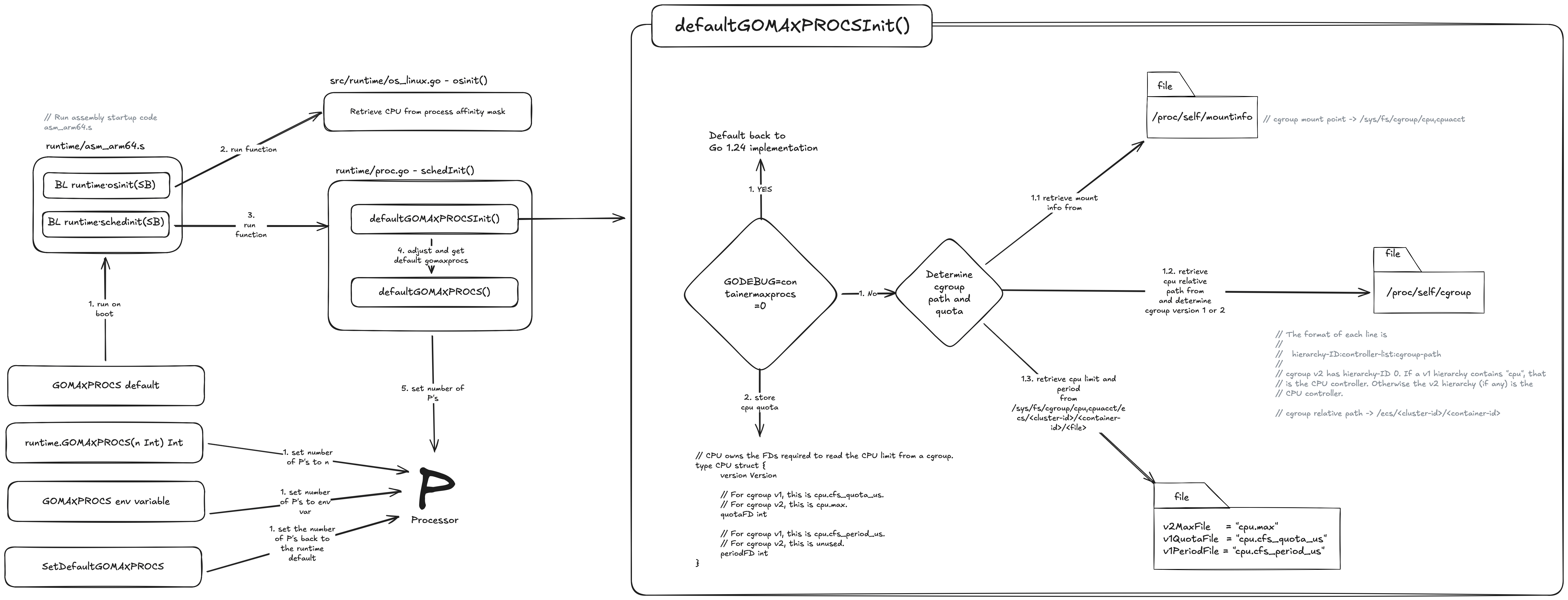
Before I dive into what is happening here I’ve outlined the main execution path for setting GOMAXPROCS above, there is a lot more going on under the hood but I think this flow covers the bulk of it.

So lets dive into the first part of that diagram 🤿 and take a look to see what is happening!

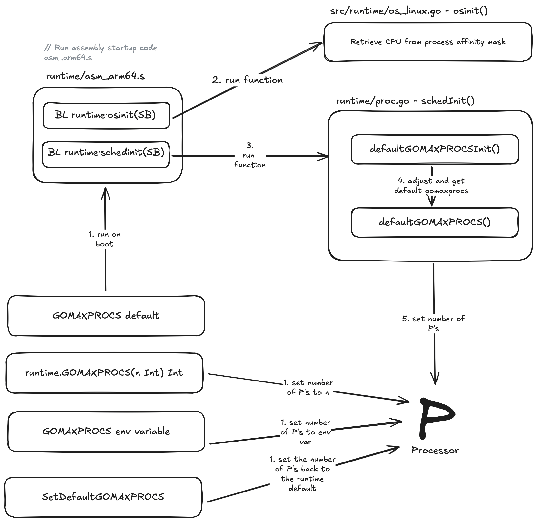
When we first run our Go application its not our main.go file which first runs like a lot of us might think (me included), It’s actually an assembly file which is specific to the architecture as set by GOARCH env variable. For example if we set GOARCH=arm64 then the assembly file that gets picked for execution is runtime/asm_arm64.s.

If we take a look at runtime/asm_arm64.s, the first piece of assembly in this file we are most interested in is:

BL runtime.osinit(SB)

Branch with Link (BL) is used to call the function runtime.osinit in runtime/os_linux.go. There are numberous OS files for different operating systems such as os_windows.go but we help guide our Go application to the correct OS file with GOOS env variable set to linux.

osinit() is responsible for retrieving the number of CPU’s from the process affinity mask. If your not familiar with a cpu affinity mask its essentially just a bit mask that allows us to bind specific processes or threads to designated cpu cores. On linux this can be achieved via the sched_setaffinity system call. This is an improvement over Go 1.24 which ignored the affinity mask and defaulted to the number of cores. So why have this here you might ask? Well in some situations we might want to allocate a single thread to a single CPU core and set the affinity mask of all other threads to exclude that CPU core we allocated the thread to. This would ensure maximum execution speed for that thread and then save the added performance cost of cache invalidation when you switch one thread off a core and onto a different core.

The second and final piece of assembly we are interested in is:

BL runtime.schedinit(SB)

Here Branch with Link (BL) is used to call the schedInit() function in runtime/proc.go which then internally runs a function called defaultGOMAXPROCSInit(). Lets take a look at the second part of that diagram now from earlier.

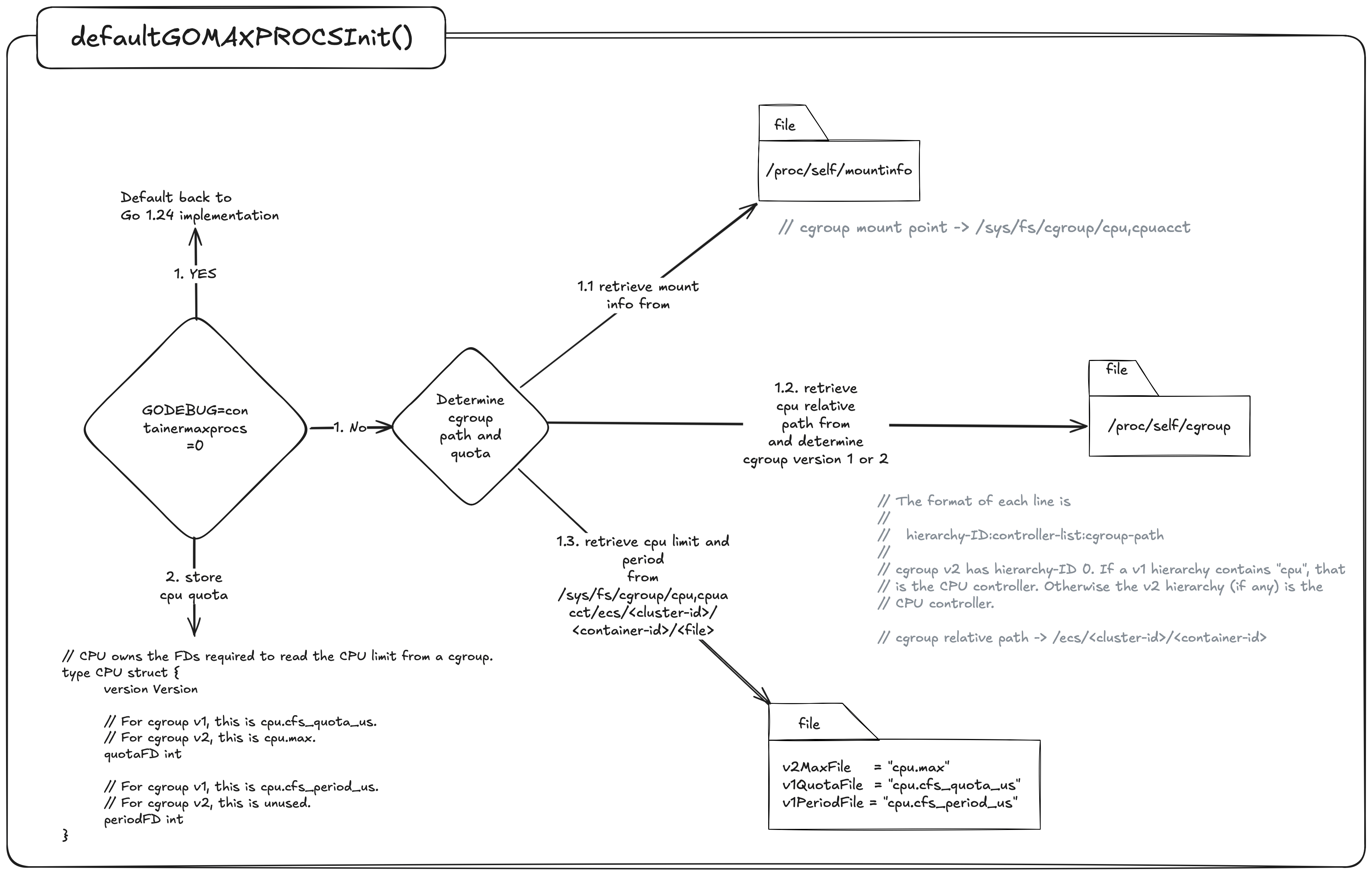
If we have the following environment variable set GODEBUG=containermaxprocs=0 Then we default back to Go1.24 implementations which will call runtime.NumCPU() to set the value for gomaxporcs. If not then we need to determine if there are any cpu limits imposed by the Completely Fair Scheduler.

To do this first we need to look up the cgroup mount point in /proc/self/mountinfo and the cpu relative path and version from /proc/self/cgroup.

To help explain how this works lets run a container on our laptop with the docker cpu resources set to 8 and the container set to a limit of 4.

// docker-compose.yml

services:
  app:
    container_name: demo
      build:
        context: .
        dockerfile: Dockerfile
    image: demo
    deploy:
      resources:
        limits:
          cpus: "4" # limit to 4 CPU

Lets first take a look at the relative path in /proc/self/cgroup to see what we get:

0::/

Ok, its just a /.

Now let have a look in /proc/self/mountinfo which will help tell us the mount point and cgroup version.

634 633 0:34 / /sys/fs/cgroup ro,nosuid,nodev,noexec,relatime - cgroup2 cgroup rw

This line in the mountinfo tells me the cgroup version is V2 by cgroup2 and the mount point is /sys/fs/cgroup.

We can now join the mount point + relative path + file based on cgroup version.

/sys/fs/cgroup + / + cpu.max

If we now cat this file:

cat /sys/fs/cgroup/cpu.max

// 400000 100000

The number on the left is the quota and the right is the period.

Now for some basic math:

400000 / 100000 = 4 cpu

and presto 🪄 ✨ we have our 4 CPU’s as expressed in our docker-compose.yml file. If this was Go 1.24 that would have been 800000 / 100000 = 8 cpu 🙅‍♂️.

Lastly Go then compares the cpu limit we derived from above to the cpu affinity mask and adjusts the gomaxprocs via adjustCgroupGOMAXPROCS() function.

Few things to note here:

1. If the cpu limit is set to 1 but the node we are running on has more than 1 core then gomaxprocs defaults to 2 not 1. Uber/automaxprocs would respect this and use 1. Not a fan of this approach as discussed earlier with CPU Limit throttling but this does help some workloads that are burstable.
2. If we are using partial limits we take the ceil. Uber/automaxprocs would floor this value.

Point 2 is an interesting one because GOMAXPROCS does not have the concept of a fractional CPU so we have to decide do we round up or down . Either way it’s a tradeoff between low-level throttling with Ceil or underutilisation of the cpu with Floor. A bit of history Uber/automaxprocs originally started with Ceil but later changed to Floor as their default implementation Issue #13. The main cause for this was because users who were setting fractional units as a buffer for other OS related tasks not tied specifically to your Go program might have needed this added fractional cpu. Approximately 6 years later after Uber decided to floor gomaxprocs they introduced RoundQuotaFunc() as a way to give the developer control over how they wanted to convert the cpu quota ie: round up/down.

Wrap Up

If you take away one thing from this, let it be that Uber/automaxprocs and Go’s 1.25 container aware Gomaxprocs implementation are not a one-size-fits-all solution 👠. These tools and implementations are designed to cater to the vast majority of workloads and do not cater to every specific use case.

If you are fine-tuning for tail latency, you must move past the surface level and look “under the hood” to understand the underlying nature of the system. Think of a master sculptor: they do not simply strike the stone; they understand the planes of the marble and how the tip of the chisel when striked against the grain gives a different outcome based on the angle they strike. They know exactly how much material to remove to reveal the form without compromising the structural integrity of the whole.

Similarly, when you master how the Go scheduler interacts with the OS and the underlying hardware, you stop just writing code but begin sculpting for performance. You learn to treat CPU quotas and scheduling latencies as your raw medium, carving out the excess medium leaving behind a lean and high-performant masterpiece.

In Part 2, I will build upon these concepts and dive into the specific tools and approaches we can use to fine-tune our Go applications. I hope to see you there ✌️

A bit about the art

All art was made using a combination of self made svg’s, along with svgs from svg repo and the go.dev site which were then altered and combined with custom self made assets on sketch and excalidraw.

References

• Operating Systems: How Linux does CPU Scheduling
• CPU Scheduling Basics
• GitHub Issue #73193
• Automaxprocs Pull Request #79
• Automaxprocs Pull Request #79
• Go 1.25 Release Notes
• Ardanlabs Go Training
• CPU Clock Speeds Explained
• The Clock Cycle of a CPU
• Kubernetes V1 CPU Shares to V2 CPU Weight
• Operating System Vs Kernel
• Linux Select Poll & Epoll
• Go epoll/kqueue
• Go syscall_linux.go
• Runtime netpoll_epoll
• What is P99
• Amazon 100ms added page load time
• Multi Threading Models
• Go stack
• Linux epll_ctl
• Uber/automaxprocs
• New async I/O API
• Kernel io_uring
• Linux Kernel Programming CPU Scheduling
• SVG Repo
• Go runtime2